multilayer perceptron
Table of Contents
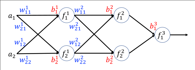
 multiplayer perceptron is a layered architecture of neurons, where:
- neurons are divded into layers
- adjacent layers are interconnected
- the notion of of \(a_0\) in is replaced with
bias
1. algorithm
1.1. instant state
good old linear combination
- forward propagation
- from input, calculate instant states and outputs of each layer, and use the outputs as input of the next layer, until the last one
1.2. output
- activation function
- a lot of choices
- identity
- \(X = f(x) = x\)
- sigmoid
- $X = f(x) = $
1.3. error
- output error
- \(\frac{1}{2} \Sigma^m_{j=1}(t^k_j-X^k_j)^2\)
- performance on Data set D
- sum of output error on each input entry
- MLP error function
- sum of output error on each input entry, in the training stage. As data don’t change, the error function is a function on weights, which are to be optimized \[ E = E(W) \]
1.4. performance
1.5. training
1.5.1. gradient decent
As error function is a \(E(W)\), with gradient decent, we can determine a proportion of adjustment to all of the individual weights(a vector of values), if applied the same time(times -1), should bring the error function down the rapidest
The gradient determined of \(E(W)\) contains all \(\Delta w\) s
1.5.2. weight update
follows the idea of gradient decent, \(\Delta w = -C \frac{dE}{dw}\) (for respective weight)
1.5.3. backpropagation ATTACH
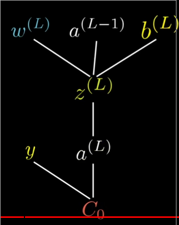
determining derivative of a specific weight/bias using chain rule, from output layer, one layer back at a time.
- using chain rule
- derivative of f(g(x)) with repect to x = f’(g(x))*g’(x) As error function is recursively calling linear combination and activation function with no additional multiply/log-like term, the derivitive is pretty much just multiplying intermediate computation varaibles, like the weight, instant state of a neuron, etc.
- one layer back at a time
- this is because a neuron may contribute to error via multiple paths, and those derivatives has to be aggregated.

- the algorithm
- Use \(\frac{dE}{da^{\text{level}}_{k}}\) as intermediate shorthand.
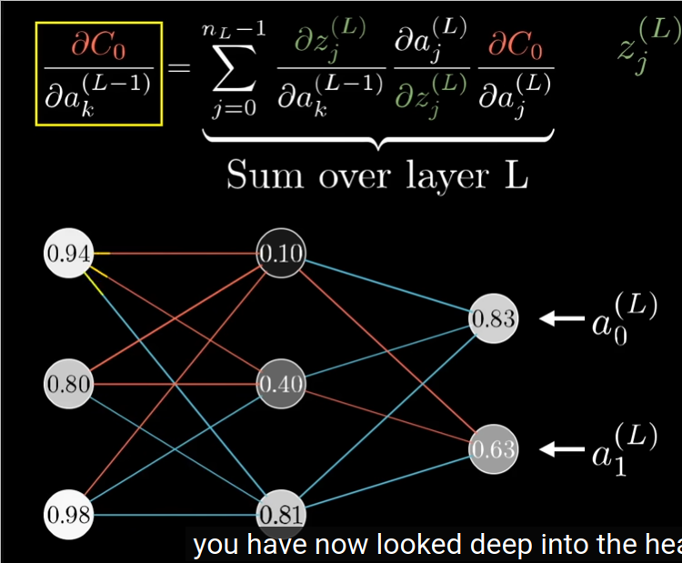
- calculating \(\frac{dE}{da^{\text{level}}_{k}}\)
starting from the closest uptream \(\frac{dE}{da^{\text{level}}_{k}}\):
- if no such upstream, then is at output layer, where it is simple \(label - output\)
- otherwise, the formula is follows:
\[ \Delta a^{l-1} = \frac{dE}{da^(l)} \frac{d\text{activation}}{d\text{instant state}} \frac{d\text{instant state}}{da^{l-1}} \]. so the same as the weight, only that the last term is now \(w_l\) instead of \(a^{l-1}\), as they multiplied as the term in the linear combination towards the instant state.
plus, \(\frac{dE}{da^{\text{level}}_{k}}\) from all possible paths has to be added together. so if a neuron in a hidden layer gives its output to 2 neurons in the next layer, it’s \(\frac{dE}{da^{\text{level}}_{k}}\) will be \(\Delta a^{l-1}\) calculated from both paths added together, as with the formula above, only 1 path is calculated at one time.
- calculating weight
 The forumla is:
\[
\Delta w^l = \frac{dE}{da^(l)} \frac{d\text{activation}}{d\text{instant state}} frac{d\text{instant state}}{dw^l}
\].
of the 3 terms:
- \(\frac{dE}{da^{l}}\) is already computed for hidden layers, and trivial for last layer (\(label_i - a^{last}_i\))
- \(\frac{d\text{activation}}{d\text{instant state}}\) is easy, as activation function’s derivative is easy, and instant state is already computed in the forward propagation.
- \(\frac{d\text{instant state}}{dw^l}\) is easy as map from \(w_l\) to the instant state is a linear combination, and the derivative of \(w_l\) to instant state is the output from last layer \(a^{l-1}\) that is coupled with \(w_l\).
starting from the closest upstream(from the direct higher layer) \(\frac{dE}{da^{\text{level}}_{k}}\), and multiply it with the activation function derivative (uses instant state), and the matching last layer input of the weight \(a^{(level - 1)}\), as instant state is computed with \(S = w_1a^{(level-1)}_1 + w_2a^{(level-1)}_2 +... + w_na^{(level-1)}_n\), of which all terms other than the \(w_ia^{(level-1)_i}\) that we are looking at can be ignored.
2. continuous and differentiable activation function
People want that so that we can calculate gradient of error function.
Here are some choices:
- generic sigmoid
\[
f(S) = \frac{\alpha}{1 + e^{-\beta S + \gamma}} + \lambda
\]
- tuning
- \(\alpha \beta\) determine steepness
- \(\beta\) determine slope
- \(\gamma\) determine x-axis shift
- \(\alpha,\lambda\) determine value range in x and y
- derivative \[ f'(S) = \frac{df}{dS} = \frac{\beta}{\alpha}(f(S)+\lambda)(\alpha + \lambda - f(S)) \]
- tuning
2.1. sigmoid
generic sigmoid with \(\alpha = 1, \beta = 1, \gamma = 0, \lambda = 0\) \[ f(s) = \frac{1}{1 + e^{-S}} \] \[ f'(s) = f(S)(1 - f(S)) \]
Backlinks
a neural network architecture to achieve sequence similarity mapping (map sequence A to sequence B that is similar to sequence A)
It defines several neural network modules that are mostly based on multilayer perceptron, and combine them sequentially(stacking) and in parallell(multiplexing), namely: